The first version of this article was published in the 1hive forum.
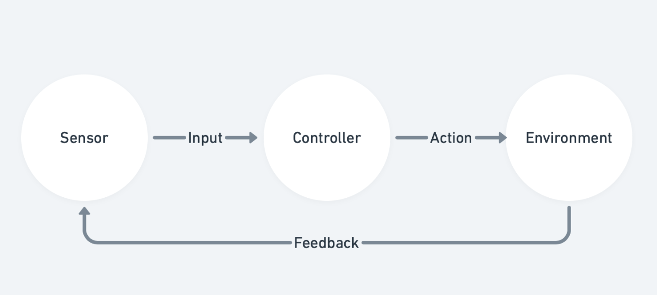
Luke once described 1hive as cybernetic superorganism, I didn't realized it was an established term in science to describe such an amazing natural phenomenon.
1hive is a decentralized autonomous organization, but that doesn't really mean very much to very many people, and even for people that are familiar with DAOs, the term has been used in so many different context that it has lost much of its meaning.
A superorganism or supraorganism is a group of synergetically interacting organisms of the same species. A community of synergetically interacting organisms of different species is called a holobiont. The term superorganism is used most often to describe a social unit of eusocial animals, where division of labour is highly specialised and where individuals are not able to survive by themselves for extended periods.
A bee hive can be considered a superorganism as well which has a very interesting way to gather information from each individual bee through quorum sensing:
Honey bees (Apis mellifera) also use quorum sensing to make decisions about new nest sites. Large colonies reproduce through a process called swarming, in which the queen leaves the hive with a portion of the workers to form a new nest elsewhere. After leaving the nest, the workers form a swarm that hangs from a branch or overhanging structure. This swarm persists during the decision-making phase until a new nest site is chosen.
The quorum sensing process in honey bees is similar to the method used by Temnothorax ants in several ways. A small portion of the workers leave the swarm to search out new nest sites, and each worker assesses the quality of the cavity it finds. The worker then returns to the swarm and recruits other workers to her cavity using the honey bee waggle dance. However, instead of using a time delay, the number of dance repetitions the worker performs is dependent on the quality of the site. Workers that found poor nests stop dancing sooner, and can, therefore, be recruited to the better sites. Once the visitors to a new site sense that a quorum number (usually 10–20 bees) has been reached, they return to the swarm and begin using a new recruitment method called piping. This vibration signal causes the swarm to take off and fly to the new nest location. In an experimental test, this decision-making process enabled honey bee swarms to choose the best nest site in four out of five trials.
Here are two "primary regulation mechanisms" for regulating bee colony behavior at the group level, and two of four or five observed mechanisms known to be used by honeybees to change the task allocation among worker bees:
By performing a waggle dance, successful foragers can share information about the direction and distance to patches of flowers yielding nectar and pollen, to water sources, or to new nest-site locations with other members of the colony.
A tremble dance is a dance performed by forager honey bees of the species Apis mellifera to recruit more receiver honey bees to collect nectar from the workers.
I have found it very interesting leaning about this and other biotic interactions, such as how trees communicate with each other using a symbiosis of their roots with the network of fungi that connect them to other trees in order to exchange sugar, water, and minerals or be aware of predatory insects. You can read more on this in:
The Social Life of Forests As a child, Suzanne Simard often roamed Canada's old-growth forests with her siblings, building forts from fallen branches, foraging mushrooms and huckleberries and occasionally eating handfuls of dirt (she liked the taste). Her grandfather and uncles, meanwhile, worked nearby as horse loggers, using low-impact methods to selectively harvest cedar, Douglas fir and white pine.
You can find the first version of this article as a hackmd published during the ETHOnline '21 hackathon.
Osmotic Funding is a protocol built on top of Superfluid Finance and Conviction Voting to create and regulate project funding streams based on the amount of interest a community gives them. Community preference is revealed continuously, since tokenholders are able to update their preferences (change their stake) at any moment.
A community of tokenholders (DAO) can use Osmotic Funding to decide which parts of the DAO should receive funding and how much. Funding proposals need a minimum amount of support to start receiving funds. Once the flow is open, they can grow or shrink over time, depending on the stake with which the token holders are supporting the proposals.
Depending on the distribution of staked tokens and the available funds in the pool, we can calculate which will be the rate of each proposal with:
r∞(i)=B⋅(1−max(T,si)T)whereT=γ⋅(s0+s1+...+sn)+T0 and B=b⋅β
The target rate (r∞) of a proposal (i) is the amount of funds a project should be receiving per second in the future.
The pool balance (b) is the amount of funding tokens that can be transmitted to grants. It will keep diminishing if there are no inflows that fund the contract at the same rate.
Max spending ratio (β) is the max percentage of the pool balance that one proposal can spend per second.
Threshold (T) is the minimum amout of staked tokens a proposal needs to start getting funded depending on amount staked on the rest of the proposals.
Threshold ratio (γ) determines the increse in the threshold for each new token staked on any proposal.
Min threshold (T0) is the minimum amount of tokens required to fund a proposal when no other proposal is being funded.
Total staked tokens (s0+s1+...+sn) are the amount of tokens that are actively voting in the protocol. It plays against a proposal if new tokens are staked on other proposals.
Staked tokens (si) are how many tokens are staked on the proposal which we calculate the rate for.
When the staked amount on a proposal (si) changes, the rate changes over time following the following formula:
rt(i)=αt⋅r0(i)+(1−αt)⋅r∞(i)
The current rate (rt) of a proposal (i) is the amount of funds per second a proposal receives in a particular instant of time (t).
The last rate (r0).
The exponential decay base (α) is a number from 0 to 1 that determines the speed in which the current rate is going to reach the target rate.
As you can see the formula has two parts. The first part starts with last rate and ends at zero over time. The second part starts at zero and grows up to target ratio over time.
Every time the target ratio changes (due to a change in token staking), we define the current ratio as the last ratio, so the rate over time can still be a continuous formula, and we reset the timer (t) to zero.
In order to know the amount of funds a proposal has accrued since the last time there was a stake change, we can calculate the definite integral of the current rate (rt) formula over time:
Because the target rate formula (r∞) does not depend on the time, we can treat it as a constant in the integral, which makes it not-so-difficult to calculate.
It calculates is the area below the curve defined by the current rate formula over time, which correspond to the amout of funds, or what is the same, the average rate (of all variations of rt(i) over the period of time) multiplied by time (t).
The first version of this article was published in the 1hive forum.
Some days ago I pointed out some inconsistencies I found in the issuance policy 1hive is using at the moment. After some days of thinking about it, I'd like to share with the community my work until now. This post has two purposes:
Propose a new issuance policy for 1hive and the rest of gardens
Educate about the process I've followed to obtain a result like this.
As the old policy, the proposed Dynamic Issuance v2 tends over time towards a particular ratio between the token balance of the common pool and the total supply (or circulating supply) of the token.
We call this ratio towards the issuance mints or burns tokens the target ratio, a number between 0 and 1.
The new issuance policy is configured using two parameters, target ratio, already used in the previous version, and recovery time, a new parameter that sets the maximum time that it cost for the ratio to recover the target percent.
The formulas that determine the ratio over time when there are no inflows or outflows on the common pool are as follow:
When we start with a ratio below the target ratio (we mint tokens into the common pool):
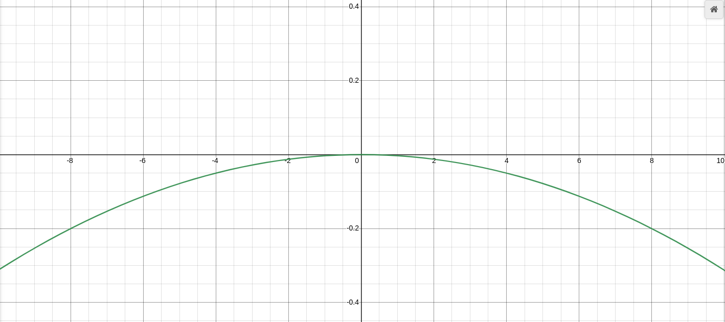
f(x)=r2−t(x−r)2+t
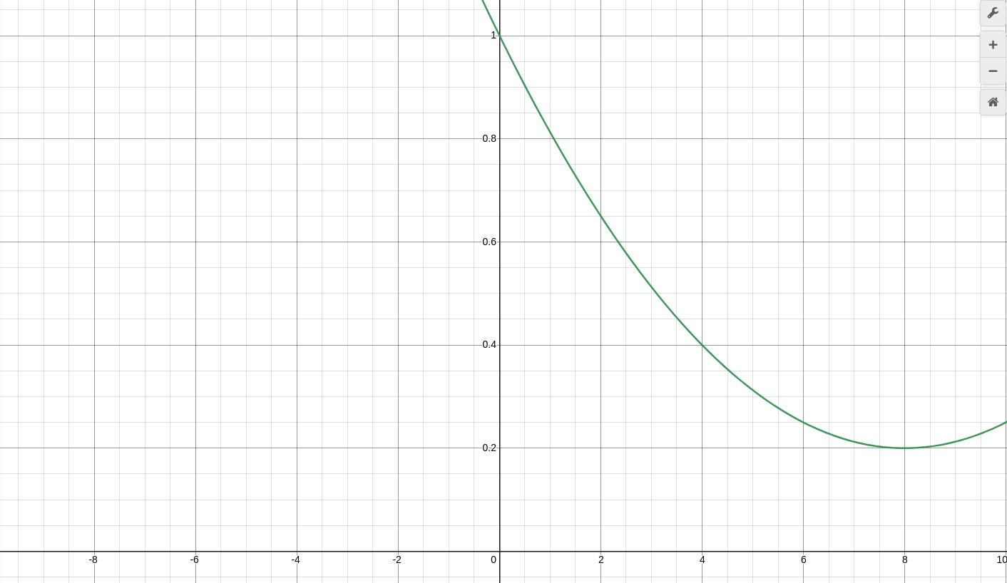
When we start with a ratio above the target ratio (we burn tokens from the common pool):
f(x)=r21−t(x−r)2+t
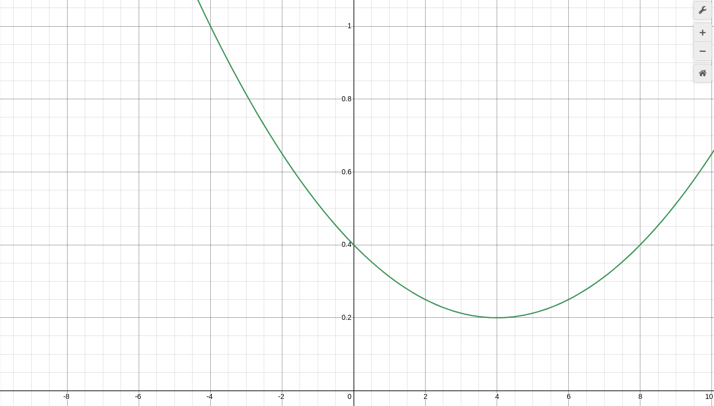
Note that both of these formulas only apply within the recovery time, after this period, the new ratio is target ratio.
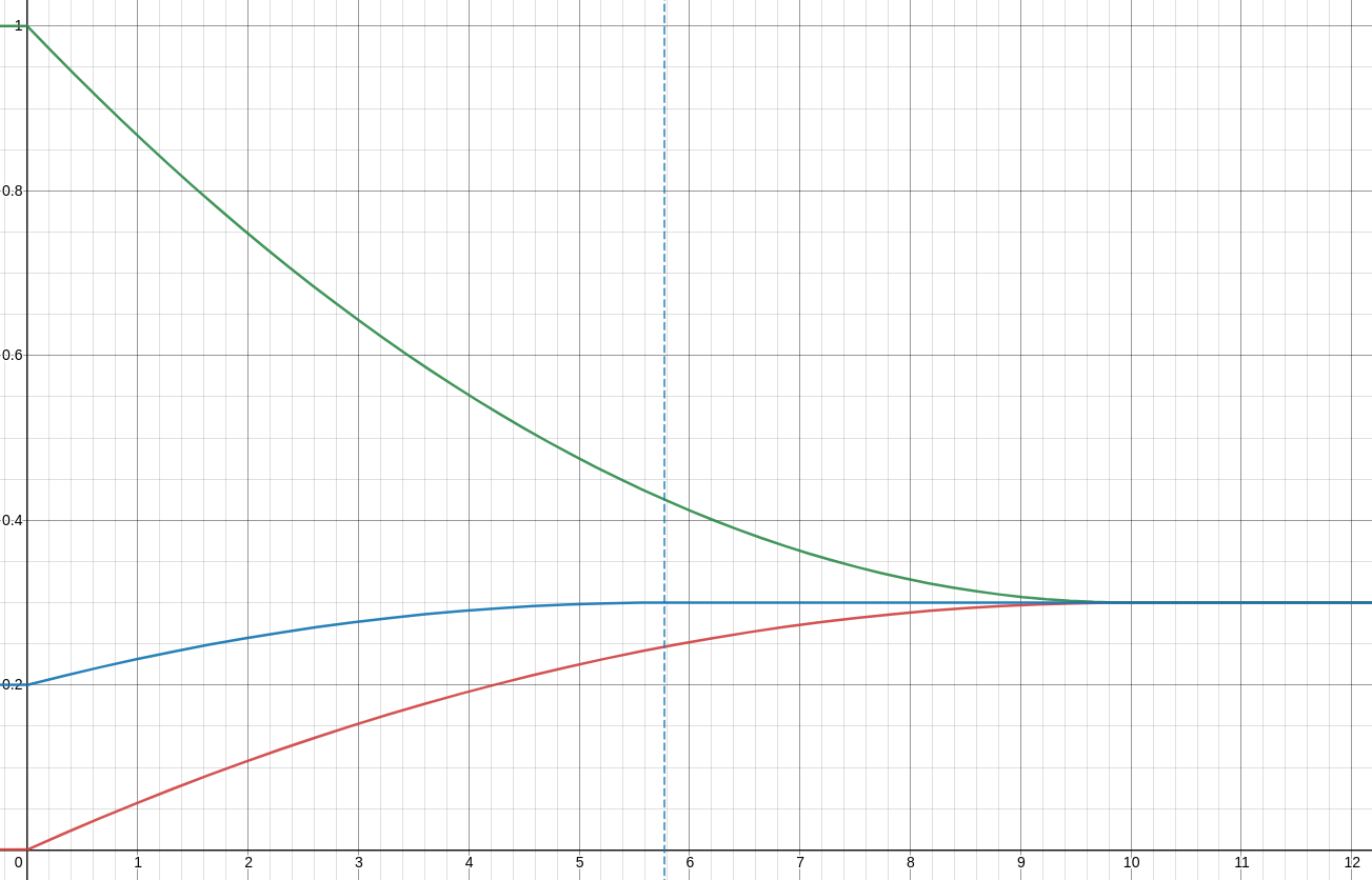
You can observe how these formulas work in this desmos. You can use target ratio to move the ratio vertically and recovery time to move the point in which curves touch each other.
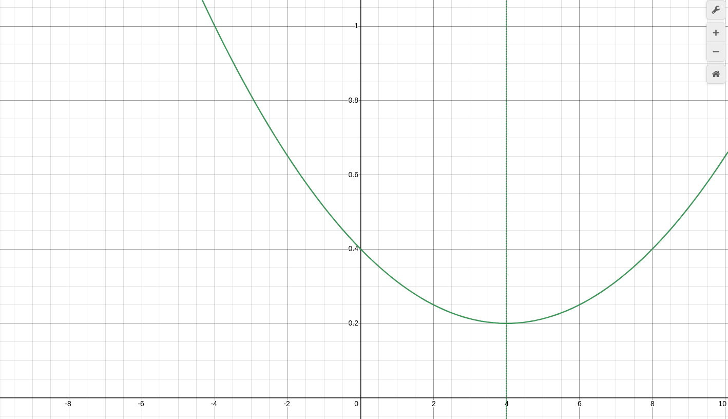
It's very unlikely that our common pool is totally full or totally empty at any point, but those equations determine the path that the ratio will travel during time starting from any point. So if we start with a ratio of 20% (current ratio), we see how the curve travels a shorter path (blue lines in the chart above).
The "blue line" formula is a bit more complex as we have to translate the equation horizontally until it matches the current ratio in the Y-axis. It is the following piecewise formula:
This can be gracefully translated to Solidity code, as we can see here (or in remix):
This is just a proof-of-concept code, the real smart contract has to actually mint or burn tokens to/from the common pool, in a similar way we were doing with the old policy (calling executeAdjustment()).
For this particular policy, we will also need to do adjustments every time that the token supply changes (some tokens are minted or burnt), or there are inflows or outflows in the common pool. This means that we will need to register the Dynamic Issuance app as a hook for the Hooked Token Manager in order to be able to act when these events occur.
I think this can be a great opportunity to explain how we can design token policies using simple math models. I recommend using desmos when you do this kind of explorations during the first stage.
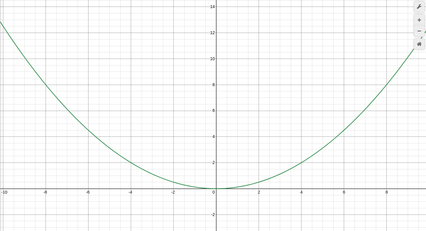
We know that we would like a curve, so we start with the formula y=x² because powers and square roots are easy to calculate in Solidity. If we divide the formula by r, we will find that the formula then passes by the points (r,r) and (-r, r).
y=r1x2
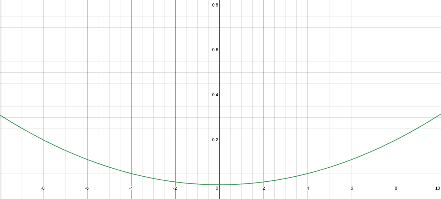
If we want it to pass by the point (r, t), which is when the recovery time (r) ends and the ratio (x) is target ratio (t), we have to divide by r again in order to obtain the point (r, 1), and by t to obtain (r, t):
y=r2tx2
We now have a formula that passes by the points (0,0) and (r, t), but it doesn't have the shape that we want, as it should decrease it's speed of emission of tokens as it reaches the target goal instead of increasing it.
In order to solve that issue we are going to apply some geometrical transformations. We will first flip the chart upside down and then we will move the entire chart from point (0, 0) to point (r, t). To flip the chart we just have to multiply the formula by -1:
y=−r2tx2
And to move the maximum of the formula, currently at point (0, 0), into the point in which recovery time has passed and we reach the target ratio(r, t), we can do a simple translation, substracting r from x and t from y:
y=−r2t(x−r)2+t
The "deflationary" formula can be obtained by replacing the -t factor by 1-t. It inverts the shape of the formula again because 1-t is positive (knowing that t≤1), and we want the formula go from 1 to t so its height must be 1-t:
In order to shift the formulas to the left until they touch the point (0,c) so we start at time 0 with a specific ratio (c). When you need to work with equations, Wolfram Alpha is your friend.
We isolate x from the "inflationary" formula and we obtain the following result:
x=trt−rt2−t⋅f(x)
We then add on the left side a shift to the point in which f(0)=c, and then solve f(x-c):
We also have to take into account that recovery time is going to be less, since we are not starting from 0% or 100%. We have to calculate where the global maximum and minimum of the formulas are in order to avoid going backwards.
The maximum of the pristine "inflationary" formula is r, as it is how we defined it from the beginning. The maximum of the "left-shifted" "inflationary" formula can be found equating it's first derivative to 0.
After defining the formula, it was straightforward to write the Solidity code for it. The only think I had to take into account is that ratios are scaled with a factor of 10^10 in order to be able to operate with Solidity (the language has no native support for decimals).
So when I was dealing with the ratios in the code you have to remember that, and use RATIO_PRECISION constant instead of 1 to do the calculations.
Also the use of fixed point arithmetic could interfere with the function _sqrt(uint256 y) but we have been lucky and all the square roots we needed to do where already multiplications of two ratio-scaled factors, so the result was also ratio-scaled.
This post has presented a piecewise formula to model the proposed Dynamic Issuance Policy v2, alongside with a proof-of-concept Solidity smart contract. I think it is a considerable improvement in respect to the previous version, but I would love to hear the comments of the community members 🐝 in order to go forward with the proposal.
This post has also been useful to explain in a detailed way the process of obtaining the formula. Hopefully this method can be replicated in the future by other token engineers to create similar policies, not only for token issuance but also for other endeavours. I hope it becomes a helpful resource in the process of designing and implementing of a token policy from its inception to the functional code.
Edited 3rd August, 2021: @divine_comedian helped me clarify some terms that were a bit opaque in the first version.